How Neural Networks Learn

Why this matters

Neural networks can look mysterious because they contain many weights and many layers. The core training idea is still the same as in simpler machine-learning models:

make prediction -> measure error -> adjust weights -> repeat

This lesson connects the older perceptron and ADALINE ideas to modern neural-network training: gradient descent, forward propagation, backpropagation, and learning rate.

Mental model

Think of a neural network as a machine with many adjustable knobs.

• The knobs are weights and biases.
• The machine makes a prediction.
• The loss function tells us how bad the prediction was.
• Gradients tell us which way to turn each knob.
• Backpropagation computes those gradients efficiently.
• Gradient descent uses the gradients to update the knobs.

Training is not the network "understanding" the data in a human sense. Training is repeated loss reduction.

Core ideas

• A neuron computes a weighted sum of inputs, adds a bias, and passes the result through an activation function.
• A perceptron uses a hard threshold for classification.
• ADALINE uses a continuous linear activation during learning, which makes loss minimization smoother.
• A loss function measures prediction error.
• Gradient descent updates parameters in the direction that reduces loss.
• Stochastic gradient descent updates from smaller pieces of data instead of the full dataset.
• Forward propagation computes predictions from inputs.
• Backpropagation computes how much each weight contributed to the loss.
• The chain rule is the calculus tool behind backpropagation.
• The learning rate controls the size of each update step.

Walkthrough

From perceptron to neural networks

The perceptron is an early supervised learning model. It receives input features, multiplies them by weights, adds a bias, and applies a threshold.

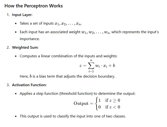
Plain version:

weighted sum = input_1 * weight_1 + input_2 * weight_2 + ... + bias

if weighted sum is large enough:
    predict class 1
else:
    predict class 0

The perceptron can learn simple linear decision boundaries. Its limitation is that the hard threshold gives a rough learning signal: the model knows whether it was wrong, but the update is not based on a smooth loss curve.

ADALINE and continuous loss

ADALINE stands for Adaptive Linear Neuron. The key difference from the perceptron is that ADALINE updates weights using a continuous output before applying the final threshold.

That matters because a continuous output allows a continuous loss function.

For mean squared error, the idea is:

loss = average of (true value - predicted value)^2

If the prediction is close to the true value, the loss is small. If the prediction is far away, the loss is large.

This is one of the big conceptual moves in supervised machine learning:

learning = finding weights and biases that minimize a loss function

What the weights mean

Weights control how strongly each input contributes to the next computation.

For a simple neuron:

input:      [x1, x2, x3]
weights:    w1, w2, w3
bias:       b

score = x1*w1 + x2*w2 + x3*w3 + b

If w2 is large, then x2 has a strong influence. If w2 is near zero, then x2 barely matters. If w2 is negative, larger x2 pushes the score down.

Bias shifts the score independently of the input values.

Digit recognition example

The slides use handwritten digit recognition as the main mental example.

Each image has 28 by 28 pixels:

28 * 28 = 784 input values

A simple network might have:

784 input neurons
16 hidden neurons
16 hidden neurons
10 output neurons

The 10 output neurons correspond to the digit classes 0 through 9.

The number of trainable values can grow quickly:

first layer weights:   784 * 16
second layer weights:   16 * 16
output layer weights:   16 * 10
biases:                 16 + 16 + 10

That gives 13,002 trainable parameters in this small example. Real networks can have millions or billions.

Gradient descent

Gradient descent is the standard update idea:

1. Compute the loss.
2. Compute the gradient of the loss with respect to each parameter.
3. Move each parameter a small step in the opposite direction of its gradient.
4. Repeat.

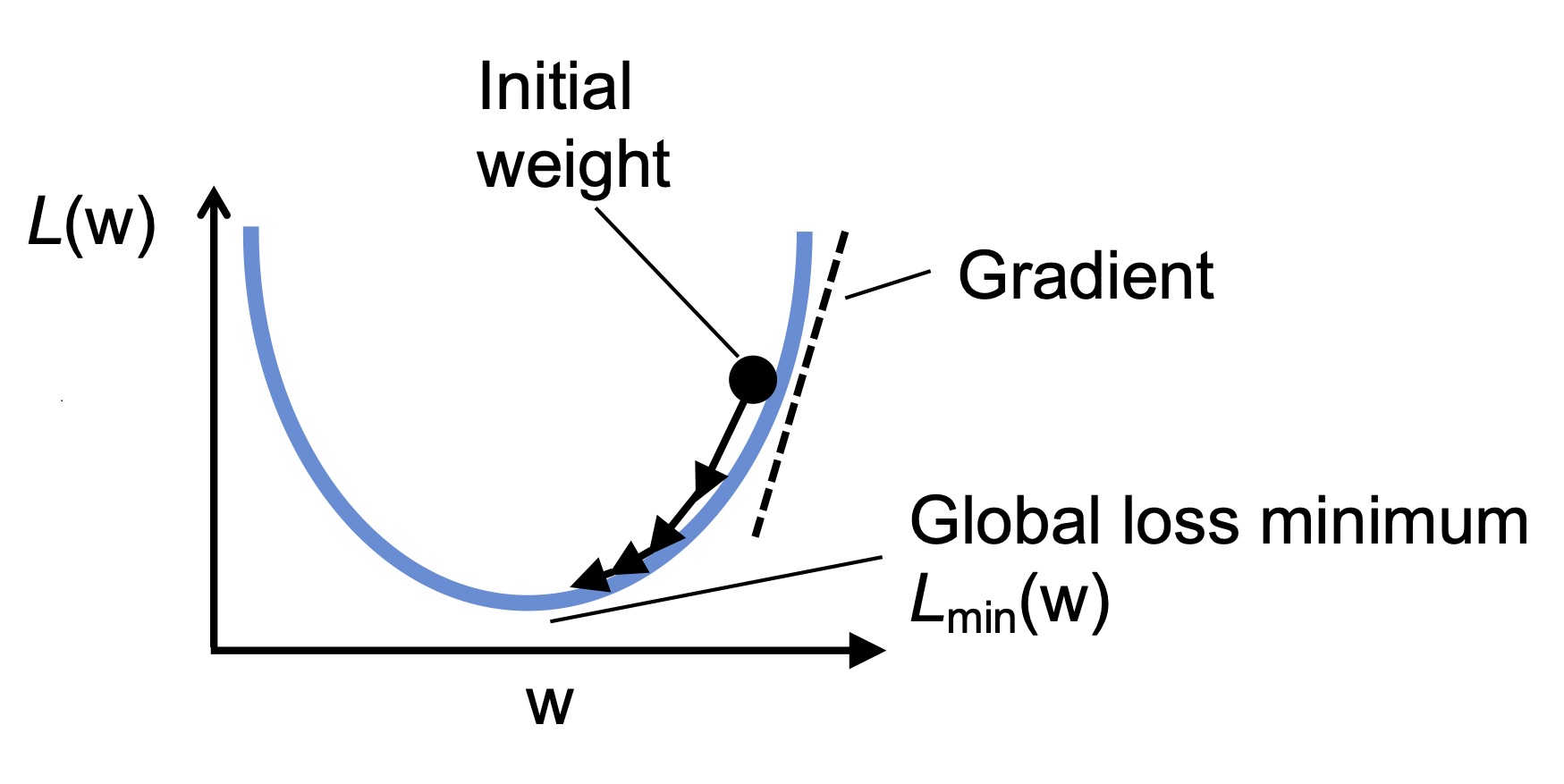
The gradient tells us the direction of steepest increase. Since we want to reduce loss, we move against it.

Plain update rule:

new weight = old weight - learning_rate * gradient

The same idea applies to biases.

Why the learning rate matters

The learning rate controls step size.

If it is too small:

training is stable but slow

If it is too large:

training may jump around, overshoot good values, or fail to converge

So the learning rate is not a detail. It determines whether gradient descent makes steady progress.

Batch, stochastic, and mini-batch gradient descent

The slides mention stochastic gradient descent because full gradient descent can be expensive on large datasets.

Three common versions:

• batch gradient descent: update using the whole training set
• stochastic gradient descent: update using one example at a time
• mini-batch gradient descent: update using a small batch of examples

Mini-batches are the practical default in deep learning. They are faster than full-batch training and less noisy than one-example-at-a-time updates.

Forward propagation

Forward propagation means computing the prediction.

For each layer:

incoming activations -> weighted sums -> activation function -> outgoing activations

The output of one layer becomes the input to the next layer.

For a classifier, the final layer produces scores or probabilities. The loss compares those predictions with the true labels.

Activation functions

Without activation functions, stacking layers would mostly collapse into one big linear model. Activation functions introduce nonlinearity, which lets neural networks learn more complex patterns.

The slides mention sigmoid:

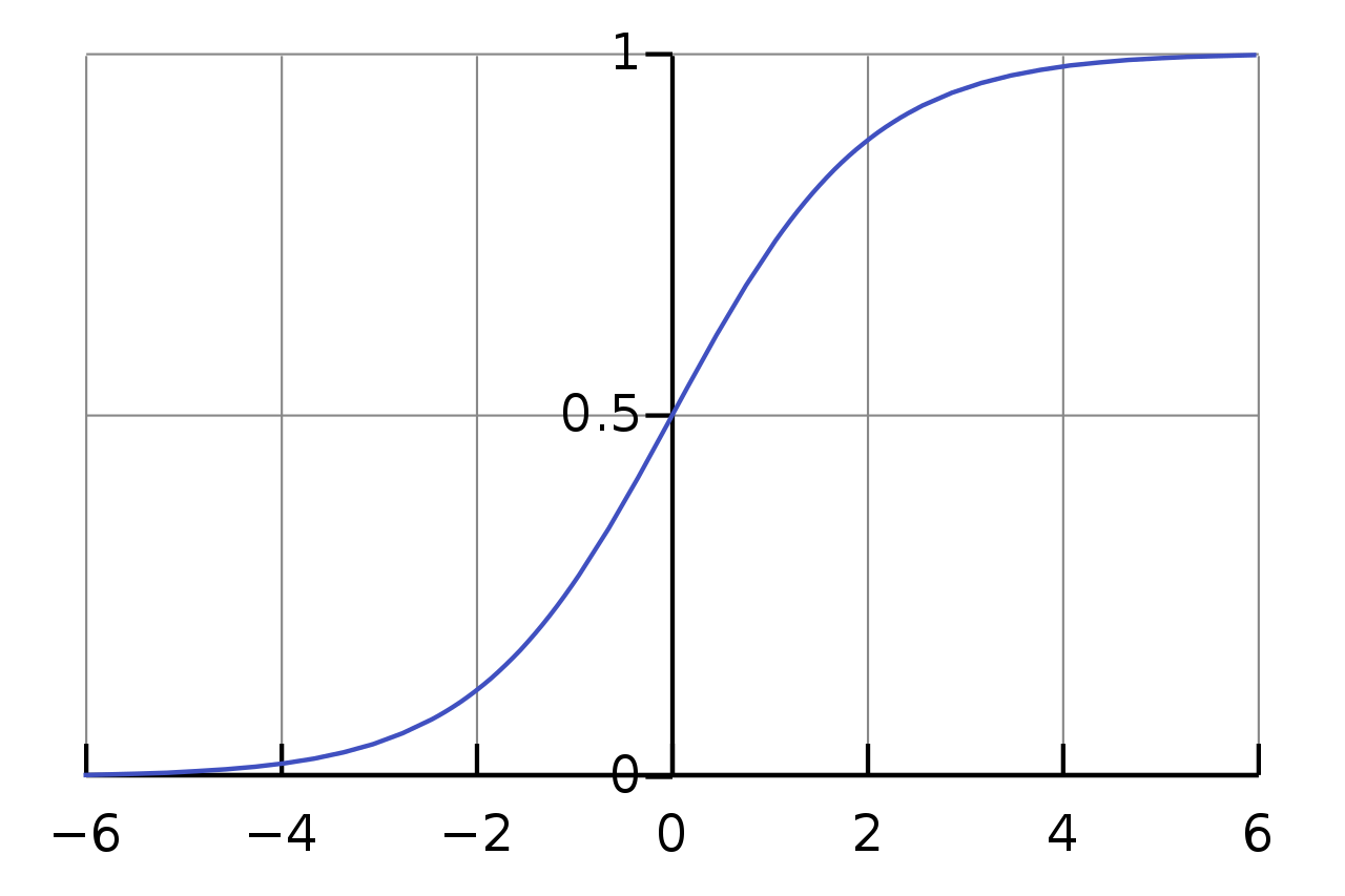
Sigmoid maps values into a smooth range between 0 and 1. It is useful for explaining neural networks historically, but modern hidden layers often use ReLU-like activations because they train better in many deep networks.

Backpropagation

Backpropagation is the efficient way to compute gradients for all weights and biases in a multilayer network.

It works backward from the loss:

loss -> output layer -> hidden layer -> earlier hidden layer -> input-side weights

At each step, it asks:

How much did this parameter contribute to the final loss?

Then gradient descent uses those answers to update the parameters.

Backpropagation is not a separate learning rule from gradient descent. It is the method for computing the gradients that gradient descent needs.

Why the chain rule matters

A neural network is a chain of computations:

input -> layer 1 -> layer 2 -> output -> loss

The chain rule tells us how a change early in the chain affects something later in the chain.

Backpropagation applies the chain rule from right to left. This reverse direction is efficient because each intermediate gradient can be reused as the computation moves backward through the layers.

This is why modern libraries such as PyTorch can train large networks: they build a computation graph during the forward pass and use automatic differentiation to compute gradients during the backward pass.

One training loop

A simplified neural-network training loop looks like this:

for epoch in range(num_epochs):
    predictions = model(X_batch)       # forward pass
    loss = loss_fn(predictions, y_batch)

    loss.backward()                    # backpropagation
    optimizer.step()                   # gradient descent update
    optimizer.zero_grad()              # clear old gradients

What this teaches:

• model(X_batch) computes predictions.
• loss_fn measures error.
• backward computes gradients.
• step updates weights and biases.
• zero_grad prevents old gradients from accumulating into the next update.

Common traps

Do not confuse backpropagation with the whole training process

Backpropagation is the gradient-computation part. Training also includes forward passes, loss calculation, parameter updates, and repeated data batches.

Remember that gradient descent moves opposite the gradient

The gradient points uphill toward increasing loss. Gradient descent subtracts it to move downhill.

Do not blame the architecture before checking the learning rate

A learning rate that is too large can make training unstable even when the model structure is fine.

Do not treat hidden-layer activations as magic

They are transformed feature representations learned from data.

Do not ignore bias terms

Biases let neurons shift activation thresholds independently of the input weights.

Do not assume neural-network loss surfaces are simple bowls

Multilayer networks can have complex, non-convex loss surfaces.

Check yourself

What are weights and biases responsible for?

Weights control how strongly inputs influence later computations. Biases shift neuron scores independently of the input values.

Why is a continuous loss function useful for learning?

It gives a smooth signal about how wrong the model is, which allows gradients to guide weight updates.

What does the gradient tell us?

It tells us the direction in parameter space where the loss increases fastest.

Why does gradient descent subtract the gradient instead of adding it?

The gradient points uphill. Subtracting it moves the parameters downhill, toward lower loss.

What is the difference between forward propagation and backpropagation?

Forward propagation computes predictions. Backpropagation computes gradients that explain how parameters contributed to the loss.

Why is the chain rule needed in multilayer networks?

Each layer depends on earlier layers. The chain rule connects those dependencies so we can compute how earlier weights affect the final loss.

What can go wrong if the learning rate is too large?

Updates can overshoot good parameter values, causing unstable training, oscillation, or failure to converge.

In a PyTorch-style loop, why do we call zero_grad?

PyTorch accumulates gradients by default. zero_grad clears old gradients so the next update uses only the current batch.

Source anchors

This lesson rewrites the main ideas from 09a-How NNs Learn.pdf:

• perceptron recap
• ADALINE and continuous loss
• supervised learning as loss minimization
• digit-recognition parameter counting
• gradient descent and stochastic gradient descent
• forward propagation
• backpropagation and the chain rule
• learning-rate sensitivity