Implementing a Multi-Layer NN

Why this matters

The previous lesson explained how neural networks learn. This lesson shows what that means in code by implementing a small multi-layer perceptron, or MLP, from scratch with NumPy.

The point is not that you should write production neural networks this way. The point is to see the moving parts that PyTorch will later automate:

initialize weights -> forward pass -> compute loss -> backpropagate gradients -> update weights

Once that loop is clear, high-level deep-learning libraries become much easier to reason about.

Mental model

An MLP is a stack of fully connected layers.

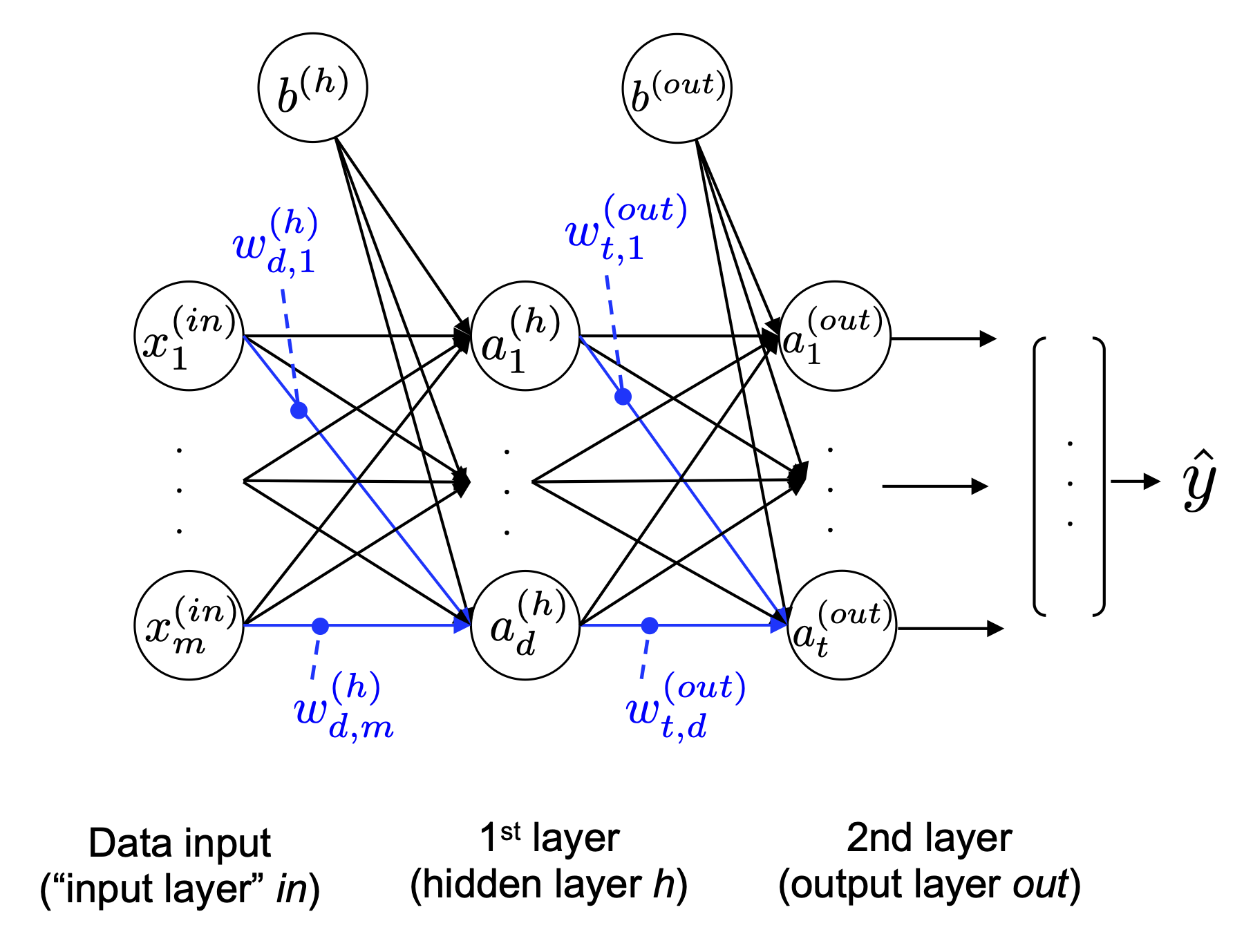
For one hidden layer:

784 pixel inputs -> hidden layer -> 10 digit outputs

Every hidden neuron receives every input feature. Every output neuron receives every hidden activation. The network learns by adjusting the weights on those connections.

Core ideas

• A multi-layer perceptron is a feedforward neural network with one or more hidden layers.
• Fully connected means every unit in one layer connects to every unit in the next layer.
• MNIST images are 28 by 28 pixels, flattened into 784 input features.
• Pixel normalization makes gradient-based optimization more stable.
• One-hot encoding represents class labels as target vectors.
• Forward propagation computes hidden activations and output activations.
• Backward propagation computes gradients for all weights and biases.
• Mini-batch training updates the model using chunks of data.
• Validation accuracy helps detect overfitting while training.
• From-scratch NumPy code teaches the mechanics, while PyTorch is the practical tool for real projects.

Walkthrough

What architecture is being built?

The notebook builds an MLP for handwritten digit classification.

The architecture is:

input features: 784
hidden units:   50
output classes: 10

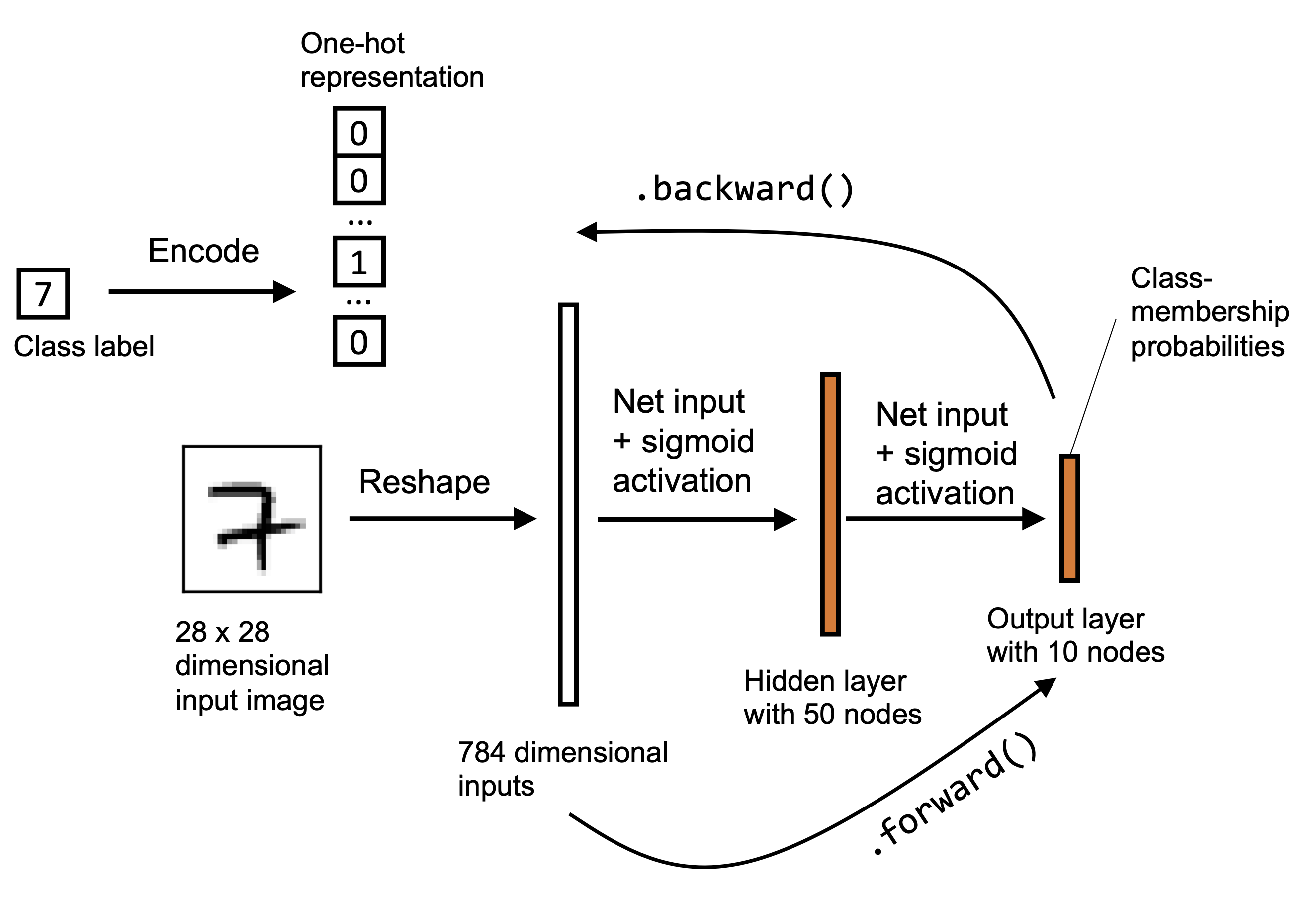
The output classes are the digits 0 through 9.

This is still a small network, but it already has many parameters:

input-to-hidden weights: 50 * 784
hidden biases:           50
hidden-to-output weights: 10 * 50
output biases:           10

Those parameters are what training updates.

Why MNIST is flattened

MNIST images are two-dimensional pictures:

28 rows * 28 columns = 784 pixels

The from-scratch MLP does not use image structure directly. It expects one feature vector per image, so each 28 by 28 image is flattened into one row with 784 values.

image matrix -> vector of 784 pixel intensities

This is simple and works reasonably well, but it discards spatial structure. Later, convolutional neural networks are designed to use that structure more directly.

Normalizing pixel values

Raw MNIST pixels range from 0 to 255. The notebook rescales them into a roughly centered range:

X = ((X / 255.0) - 0.5) * 2

That maps:

0   -> -1
127 -> about 0
255 -> 1

Why this helps:

• gradients are usually more stable
• weights do not need to compensate for huge input values
• optimization tends to behave better

Train, validation, and test split

The notebook separates the data into:

• training set: used to update weights
• validation set: used to monitor model choices during training
• test set: used at the end to estimate generalization

The important discipline is:

train on training data
tune using validation data
report final performance on test data

If you repeatedly tune based on the test set, the test set stops being an honest final check.

One-hot labels

The raw label for an image might be:

7

The network has 10 output nodes, so the target is converted into a vector:

[0, 0, 0, 0, 0, 0, 0, 1, 0, 0]

This is called one-hot encoding. The correct class has value 1; all other classes have value 0.

def int_to_onehot(y, num_labels):
    ary = np.zeros((y.shape[0], num_labels))
    for i, val in enumerate(y):
        ary[i, val] = 1
    return ary

The MLP class

The notebook defines a NeuralNetMLP class with:

• __init__: initialize weights and biases
• forward: compute predictions
• backward: compute gradients

The simplified shape is:

class NeuralNetMLP:
    def __init__(self, num_features, num_hidden, num_classes):
        self.weight_h = ...
        self.bias_h = ...
        self.weight_out = ...
        self.bias_out = ...

    def forward(self, x):
        ...
        return a_h, a_out

    def backward(self, x, a_h, a_out, y):
        ...
        return gradients

This differs from scikit-learn's usual .fit() and .predict() style because the goal is to expose the neural-network mechanics.

Weight matrix shapes

Shape discipline is one of the most important practical skills in neural networks.

For this model:

X mini-batch:      [batch_size, 784]
hidden weights:   [50, 784]
hidden bias:      [50]
hidden output:    [batch_size, 50]
output weights:   [10, 50]
output bias:      [10]
final output:     [batch_size, 10]

The transpose in the dot product makes the dimensions align:

z_h = np.dot(x, self.weight_h.T) + self.bias_h

If x has shape [100, 784] and weight_h.T has shape [784, 50], the result has shape [100, 50].

Forward pass

The forward pass computes hidden activations, then output activations.

def sigmoid(z):
    return 1.0 / (1.0 + np.exp(-z))


def forward(self, x):
    z_h = np.dot(x, self.weight_h.T) + self.bias_h
    a_h = sigmoid(z_h)

    z_out = np.dot(a_h, self.weight_out.T) + self.bias_out
    a_out = sigmoid(z_out)

    return a_h, a_out

What this teaches:

• z_h is the hidden-layer weighted sum
• a_h is the hidden-layer activation
• z_out is the output-layer weighted sum
• a_out contains one score per digit class

The predicted class is the index with the largest output score:

predicted_labels = np.argmax(a_out, axis=1)

Loss and accuracy

The notebook uses mean squared error for teaching simplicity:

def mse_loss(targets, probas, num_labels=10):
    onehot_targets = int_to_onehot(targets, num_labels=num_labels)
    return np.mean((onehot_targets - probas) ** 2)

Accuracy is separate:

def accuracy(targets, predicted_labels):
    return np.mean(predicted_labels == targets)

Loss is what the optimizer directly tries to reduce. Accuracy is easier for humans to read, but it is not always smooth enough to optimize directly.

Mini-batch generator

Instead of processing all 55,000 training examples at once, the notebook uses mini-batches.

def minibatch_generator(X, y, minibatch_size):
    indices = np.arange(X.shape[0])
    np.random.shuffle(indices)

    for start_idx in range(0, indices.shape[0] - minibatch_size + 1, minibatch_size):
        batch_idx = indices[start_idx:start_idx + minibatch_size]
        yield X[batch_idx], y[batch_idx]

Why this matters:

• mini-batches reduce memory pressure
• updates happen more often than full-batch training
• matrix operations stay efficient
• shuffling prevents the model from seeing data in the same order every epoch

Training loop

The training loop ties everything together:

for epoch in range(num_epochs):
    for X_mini, y_mini in minibatch_generator(X_train, y_train, minibatch_size):
        a_h, a_out = model.forward(X_mini)
        gradients = model.backward(X_mini, a_h, a_out, y_mini)

        d_w_out, d_b_out, d_w_h, d_b_h = gradients

        model.weight_h -= learning_rate * d_w_h
        model.bias_h -= learning_rate * d_b_h
        model.weight_out -= learning_rate * d_w_out
        model.bias_out -= learning_rate * d_b_out

Read it as:

predict -> compute gradients -> step downhill

The update line uses subtraction because gradients point toward increasing loss. Training moves in the opposite direction.

Monitoring training

After each epoch, the notebook computes:

• training MSE
• training accuracy
• validation accuracy

This answers two different questions:

Is the model fitting the training data?
Is the model still performing well on data it is not trained on?

If training accuracy keeps rising while validation accuracy stalls or drops, the model is overfitting.

The notebook observes a small gap after more epochs: training accuracy becomes slightly higher than validation accuracy.

Testing and inspecting mistakes

The test set is used after training to estimate final performance.

The notebook also looks at misclassified images. That is a useful habit because aggregate accuracy does not tell you what kind of mistakes the model makes.

Example interpretation:

some handwritten 7s with a horizontal bar may be underrepresented

This is the kind of observation that can lead to better data collection, augmentation, or model choice.

Backpropagation in this notebook

Backpropagation computes gradients for:

• output weights
• output biases
• hidden weights
• hidden biases

The output layer is more direct: compare output activation with the target.

The hidden layer is less direct: hidden units influence the loss through the output layer, so their gradients must include the downstream paths. That is why the chain rule matters.

Plain version:

output layer gradient:
    how did this output weight affect the loss?

hidden layer gradient:
    how did this hidden weight affect later activations, and therefore the loss?

Why local minima are mentioned

Neural-network loss surfaces are not simple smooth bowls.

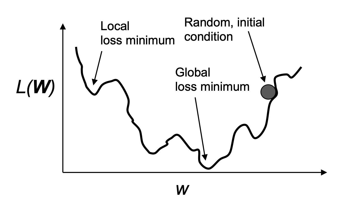
The picture is simplified, but the warning is real:

• training can be sensitive to initialization
• learning rate can be too small or too large
• deeper networks can have harder optimization problems
• modern optimizers and techniques help, but do not remove the need to monitor training

Common traps

From scratch means production-ready.

The NumPy implementation is for learning. For real neural networks, use PyTorch or a similar library.

The output scores are guaranteed probabilities.

In this teaching model, sigmoid outputs are treated like class scores. Modern multiclass classifiers usually use softmax with cross-entropy.

Accuracy is the loss.

Accuracy is a metric. The model updates weights using gradients from a differentiable loss.

The validation set is just extra training data.

Validation data should not update weights. It is for monitoring and model selection.

More epochs always help.

More epochs can reduce training loss while increasing overfitting.

Shape errors are minor syntax issues.

Neural-network code is mostly tensor shape discipline. Wrong dimensions usually mean the computation itself is wrong.

Backpropagation is only for the output layer.

Backpropagation sends gradient information backward through all trainable layers.

Check yourself

Why does each MNIST image become 784 input features?

Each image has 28 by 28 pixels, and 28 times 28 equals 784. The MLP uses a flattened vector representation.

Why normalize pixel values before training?

Smaller, centered input values usually make gradient-based optimization more stable.

What does one-hot encoding do?

It converts an integer class label into a target vector with 1 at the correct class index and 0 elsewhere.

What does the hidden layer output shape represent?

It contains one row per mini-batch example and one column per hidden unit.

Why does the training loop use mini-batches?

Mini-batches reduce memory use, keep matrix operations efficient, and allow more frequent weight updates than full-batch training.

What is the difference between loss and accuracy?

Loss is the differentiable quantity used for gradient updates. Accuracy is a human-readable metric counting correct predictions.

Why compare training and validation accuracy?

The comparison shows whether the model is learning useful patterns or starting to overfit the training data.

Why is PyTorch introduced after this notebook?

PyTorch automates gradient computation and provides practical tools for building larger neural networks, while this notebook teaches the mechanics.

Source anchors

This lesson rewrites the main ideas from 09b-Implementing a Multi-Layer NN.ipynb:

• MLP architecture and fully connected layers
• MNIST input representation
• pixel normalization
• train/validation/test split
• one-hot encoding
• NumPy implementation of NeuralNetMLP
• forward and backward methods
• mini-batch training loop
• MSE and accuracy monitoring
• validation/test evaluation and misclassified examples
• backpropagation, chain rule, and convergence remarks