Introduction to PyTorch

Why this matters

The previous lesson implemented a neural network by hand with NumPy. PyTorch gives you the same core workflow with better tools:

tensors -> computation graph -> automatic gradients -> optimizer updates

This matters because later lessons build toward language models. Those models are too large and too complex to train comfortably with hand-written NumPy backpropagation.

Mental model

PyTorch is three things at once:

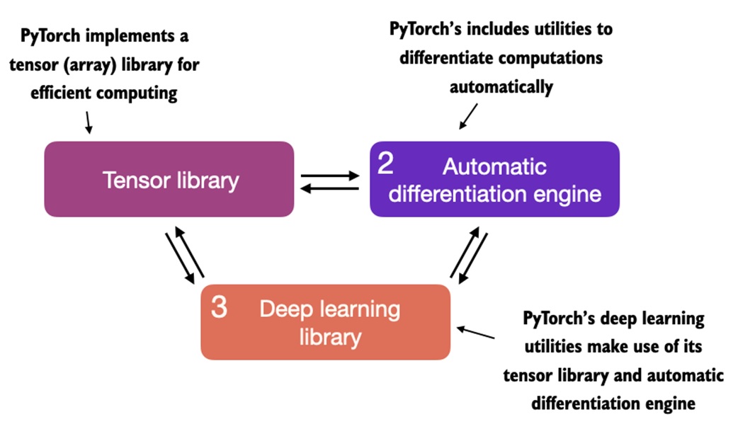
• a tensor library, like NumPy with GPU support
• an automatic differentiation engine, called autograd
• a neural-network toolkit, with layers, losses, optimizers, datasets, and training utilities

The main shift from NumPy is that PyTorch can remember tensor operations and compute gradients automatically.

Core ideas

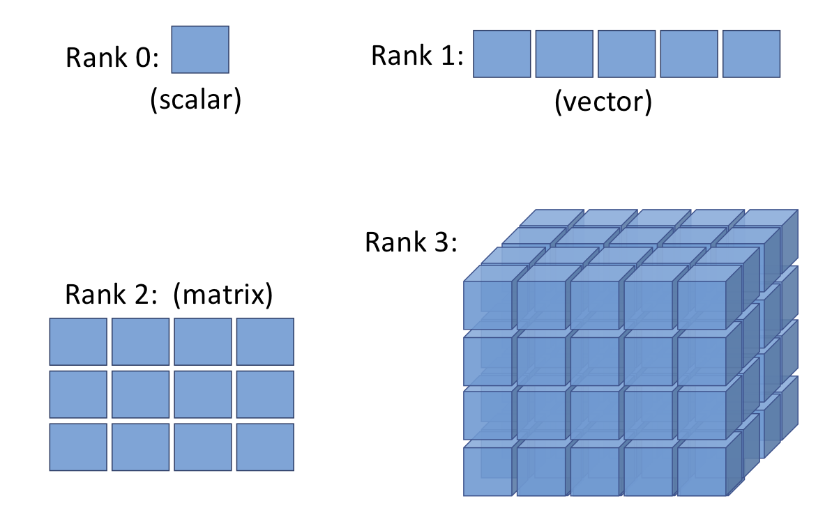
• A tensor is a numeric array: scalar, vector, matrix, or higher-dimensional block.
• PyTorch tensors can live on CPU or GPU.
• Tensor shape and dtype must match the operation you want to run.
• requires_grad=True tells PyTorch to track operations for gradient computation.
• loss.backward() computes gradients for trainable parameters.
• optimizer.step() updates parameters using those gradients.
• optimizer.zero_grad() clears old gradients before the next update.
• torch.nn.Module is the standard way to define reusable models.
• Dataset returns individual examples; DataLoader batches, shuffles, and loads them.
• During inference, use model.eval() and torch.no_grad() or torch.inference_mode().
• Save learned weights with state_dict, not by relying on a live Python object.

Walkthrough

Installing and checking PyTorch

The notebook begins with installation and GPU checks.

import torch

torch.cuda.is_available()

If this returns True, PyTorch can see a CUDA-capable GPU. If it returns False, the code can still run on CPU, just slower for larger models.

In practice, use the official PyTorch install selector for your operating system and CUDA version. The exact install command changes depending on your machine.

Tensors

Tensors generalize arrays:

0D tensor -> scalar
1D tensor -> vector
2D tensor -> matrix
3D+ tensor -> stacked numeric blocks

Create tensors from Python lists or NumPy arrays:

import numpy as np
import torch

a = [1, 2, 3]
b = np.array([4, 5, 6], dtype=np.int32)

t_a = torch.tensor(a)
t_b = torch.from_numpy(b)

Create common tensors directly:

ones = torch.ones(2, 3)
random_values = torch.rand(2, 3)

For images and deep-learning batches, a common convention is:

[batch, channels, height, width]

For text models, you will often see:

[batch, context_length, embedding_dim]

Shape and dtype operations

Most PyTorch errors are shape or dtype errors. The notebook introduces the essential tools:

t = torch.rand(3, 5)
t_transposed = torch.transpose(t, 0, 1)

t = torch.zeros(30)
t_reshaped = torch.reshape(t, (5, 6))

t = torch.zeros(1, 2, 1, 4, 1)
t_squeezed = torch.squeeze(t)

Use .to(...) to change dtype or device:

t_int64 = t_a.to(torch.int64)

Later you will also see:

features = features.to(device)
labels = labels.to(device)

That moves tensors to CPU or GPU.

Tensor math

PyTorch supports elementwise math, reductions, matrix multiplication, splitting, stacking, and concatenation.

Examples:

product = torch.multiply(t1, t2)
column_means = torch.mean(t1, dim=0)
matrix_product = t1 @ t2.T
row_norms = torch.linalg.norm(t1, ord=2, dim=1)

The pattern to watch:

dim=0 -> operate down rows, one result per column
dim=1 -> operate across columns, one result per row

For classification outputs, this is why torch.argmax(logits, dim=1) means "choose the best class for each example."

Computation graphs

PyTorch builds computation graphs from tensor operations.

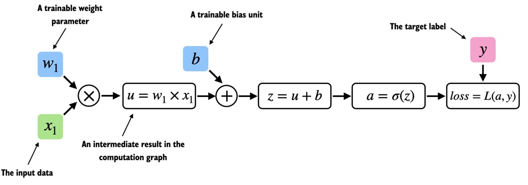
A tiny logistic-regression-like example:

import torch
import torch.nn.functional as F

y = torch.tensor([1.0])
x1 = torch.tensor([1.1])
w1 = torch.tensor([2.2], requires_grad=True)
b = torch.tensor([0.0], requires_grad=True)

z = x1 * w1 + b
a = torch.sigmoid(z)
loss = F.binary_cross_entropy(a, y)

Because w1 and b have requires_grad=True, PyTorch tracks how loss depends on them.

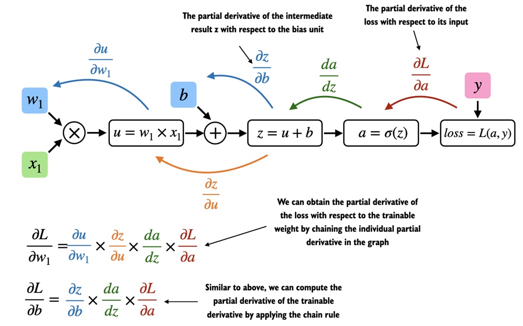
Autograd

Autograd is PyTorch's automatic differentiation system.

The usual training pattern is:

loss.backward()

print(w1.grad)
print(b.grad)

After backward, each tracked parameter stores its gradient in .grad.

That replaces the hand-written .backward() method from the NumPy MLP lesson.

Defining a model with nn.Sequential

For simple feedforward models, torch.nn.Sequential is concise:

import torch.nn as nn

model = nn.Sequential(
    nn.Linear(input_features, 30),
    nn.ReLU(),
    nn.Linear(30, 15),
    nn.ReLU(),
    nn.Linear(15, 3),
)

Important: for multiclass classification with nn.CrossEntropyLoss, the model should return raw logits. Do not add Softmax as the final training layer. CrossEntropyLoss applies the needed log-softmax internally in a numerically stable way.

Use softmax later only if you want to display probabilities:

probas = torch.softmax(logits, dim=1)

Defining a model with nn.Module

For reusable models, subclass torch.nn.Module.

class NeuralNetwork(nn.Module):
    def __init__(self, num_inputs, num_outputs):
        super().__init__()
        self.layers = nn.Sequential(
            nn.Linear(num_inputs, 30),
            nn.ReLU(),
            nn.Linear(30, 20),
            nn.ReLU(),
            nn.Linear(20, num_outputs),
        )

    def forward(self, x):
        logits = self.layers(x)
        return logits

What this teaches:

• __init__ defines the trainable layers
• forward defines how inputs flow through the model
• you normally do not implement backward
• PyTorch tracks parameters from layers such as nn.Linear

Count trainable parameters:

num_params = sum(p.numel() for p in model.parameters() if p.requires_grad)

Device handling

PyTorch tensors and models must be on the same device.

device = torch.device("cuda" if torch.cuda.is_available() else "cpu")

model = model.to(device)
features = features.to(device)
labels = labels.to(device)

If the model is on GPU but the data is on CPU, operations fail. Move both consistently.

Dataset and DataLoader

The notebook introduces PyTorch's data pipeline:

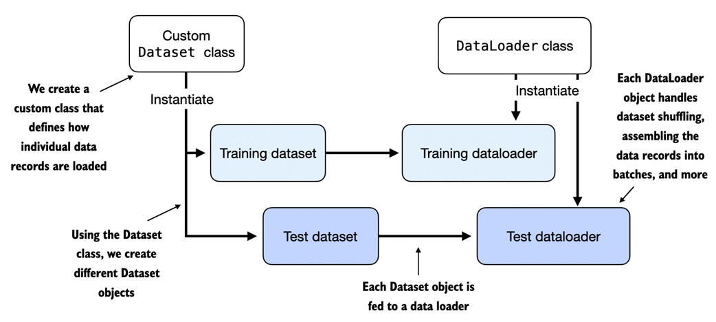
• Dataset: knows how to return one example
• DataLoader: turns examples into batches and handles shuffling

A minimal custom dataset:

from torch.utils.data import Dataset

class ToyDataset(Dataset):
    def __init__(self, X, y):
        self.features = X
        self.labels = y

    def __getitem__(self, index):
        return self.features[index], self.labels[index]

    def __len__(self):
        return self.labels.shape[0]

Wrap it in a loader:

from torch.utils.data import DataLoader

train_loader = DataLoader(
    dataset=train_ds,
    batch_size=2,
    shuffle=True,
    drop_last=True,
)

Why this matters:

• batching keeps memory use controlled
• shuffling changes example order each epoch
• drop_last=True avoids tiny final batches
• num_workers can parallelize data loading for larger datasets

Training loop

A standard PyTorch training loop has a stable shape:

import torch.nn.functional as F

optimizer = torch.optim.SGD(model.parameters(), lr=0.5)

for epoch in range(num_epochs):
    model.train()

    for features, labels in train_loader:
        features = features.to(device)
        labels = labels.to(device)

        logits = model(features)
        loss = F.cross_entropy(logits, labels)

        optimizer.zero_grad()
        loss.backward()
        optimizer.step()

Read it as:

training mode -> forward pass -> loss -> clear old gradients -> backward pass -> update

The order of zero_grad, backward, and step matters.

Evaluation and inference

For evaluation:

model.eval()

with torch.no_grad():
    logits = model(features)
    predictions = torch.argmax(logits, dim=1)

Use model.eval() because layers like dropout and batch normalization behave differently during training and evaluation.

Use torch.no_grad() or torch.inference_mode() because you do not need gradients for evaluation. That saves memory and computation.

Accuracy function

A reusable accuracy function loops over a dataloader:

def compute_accuracy(model, dataloader, device):
    model.eval()
    correct = 0
    total = 0

    with torch.no_grad():
        for features, labels in dataloader:
            features = features.to(device)
            labels = labels.to(device)

            logits = model(features)
            predictions = torch.argmax(logits, dim=1)

            correct += torch.sum(predictions == labels).item()
            total += labels.shape[0]

    return correct / total

This scales better than trying to evaluate an entire large dataset at once.

Saving and loading

The recommended basic pattern is to save the model's state_dict.

torch.save(model.state_dict(), "model.pth")

Load it into a model with the same architecture:

model = NeuralNetwork(num_inputs=2, num_outputs=2)
model.load_state_dict(torch.load("model.pth"))
model.eval()

state_dict stores learned weights and biases. The class definition still needs to exist when you load those weights.

Common traps

PyTorch tensors can hold arbitrary Python objects like NumPy arrays can.

PyTorch tensors are numeric. Text, categories, and objects need encodings, dictionaries, or embeddings.

Softmax should always be the last model layer.

For training with CrossEntropyLoss, return logits. Apply softmax only for displaying probabilities.

Calling backward() updates the model.

backward() computes gradients. optimizer.step() updates the parameters.

Gradients reset automatically.

They do not. Use optimizer.zero_grad() each update.

CPU tensors and GPU tensors can mix freely.

The model and tensors used in one operation must be on the same device.

Evaluation is just training without labels.

Evaluation should use model.eval() and no-gradient context to get correct behavior and save resources.

A DataLoader is the dataset.

The dataset defines individual examples. The dataloader defines batching, shuffling, and loading behavior.

Check yourself

What does requires_grad=True do?

It tells PyTorch to track operations on that tensor so gradients can be computed during backpropagation.

What is stored in a parameter's .grad attribute?

The gradient of the loss with respect to that parameter after loss.backward() has been called.

Why do we call optimizer.zero_grad() before loss.backward()?

PyTorch accumulates gradients by default. Clearing them prevents old gradients from affecting the current update.

What does optimizer.step() do?

It updates model parameters using the gradients and the optimizer's update rule.

Why should CrossEntropyLoss receive logits?

It combines log-softmax and negative log-likelihood internally for numerical stability.

What is the difference between Dataset and DataLoader?

A Dataset returns individual examples. A DataLoader batches, shuffles, and iterates over those examples.

Why use model.eval() during evaluation?

It switches layers such as dropout and batch normalization into evaluation behavior.

What does state_dict save?

It saves the learned parameter tensors, such as weights and biases, for the model architecture.

Source anchors

This lesson rewrites the main ideas from 11-Introduction to PyTorch.ipynb:

• PyTorch installation and CUDA check
• tensors, shape, dtype, and tensor operations
• computation graphs and autograd
• manual gradient examples with requires_grad
• simple MLPs with nn.Sequential
• reusable models with torch.nn.Module
• device handling for CPU/GPU
• Dataset and DataLoader
• PyTorch training loop
• inference, accuracy computation, and save/load with state_dict